온라인 판매 군집분석
데이터 로딩
import pandas as pd
import numpy as np

retail = pd.read_excel('./dataset/online_retail.xlsx')
print(retail.shape)
(525461, 8)
데이터 확인
retail.head()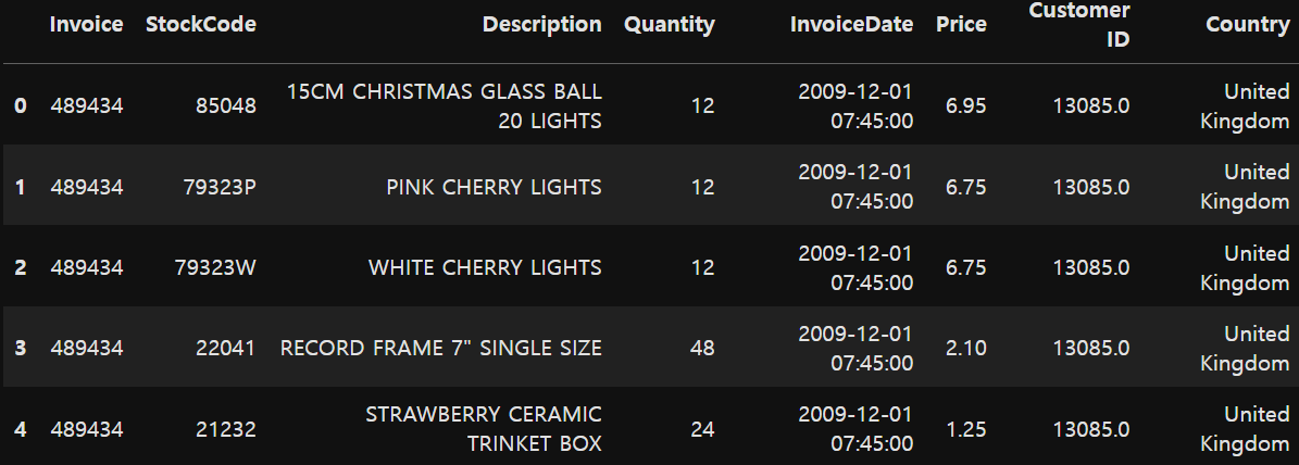
invoice : 송장 번호 / StockCode : 품목코드 / Description : 설명 / Quantity : 제품수량 / InvoiceDate : 송장 날짜 및 시간 / Price : 제품 가격 / CustomerID : 고객번호 / Country : 고객 거주 국가명
retail.info()<class 'pandas.core.frame.DataFrame'>
RangeIndex: 525461 entries, 0 to 525460
Data columns (total 8 columns):
# Column Non-Null Count Dtype
--- ------ -------------- -----
0 Invoice 525461 non-null object
1 StockCode 525461 non-null object
2 Description 522533 non-null object
3 Quantity 525461 non-null int64
4 InvoiceDate 525461 non-null datetime64[ns]
5 Price 525461 non-null float64
6 Customer ID 417534 non-null float64
7 Country 525461 non-null object
dtypes: datetime64[ns](1), float64(2), int64(1), object(4)
memory usage: 32.1+ MB몇 개의 컬럼에 결측치가 존재한다는 것을 알 수 있다.
데이터 전처리
결측치 확인 및 제거
retail.isna().sum()Invoice 0
StockCode 0
Description 2928
Quantity 0
InvoiceDate 0
Price 0
Customer ID 107927
Country 0
dtype: int64결측치 확인: 설명과 고객ID에서 결측치가 발생했다는 것을 알 수 있었다.
삭제를 한다고 해서 데이터 수의 영향이 가는 양이 아니며, 대신 채워 넣을 방법이 없기 때문에 결측치는 삭제한다.
retail = retail.dropna()
데이터 타입 변경
1. 고객번호를 정수타입으로 변경
시각적으로 보기 좋게 하기 위해 실수형 > 정수형 으로 변경한다.
retail['Customer ID'] = retail['Customer ID'].astype('int')
2. 송장번호를 정수타입으로 변경
정수타입으로 변경 전 취소 데이터 삭제 필요 (# C489449 -> 정수형으로 정상적으로 바뀔 수 없음)
retail['Invoice'] = retail['Invoice'].astype('int')retail['Invoice'].astype('int') 을 하게 되면 'C489449' 같은 취소되었다는 표시를 가진 송장번호들이 있다.
때문에 취소 주문건을 삭제하여 데이터의 유효성을 올리고 정수타입으로 변경할 수 있게 한다.
3. 취소 주문건수 확인하기
- 취소 표현 : 취소 주문건을 음수로 표현 / 위와 같이 C 를 통해 송장 번호에 표시
두 가지 표현방식을 확인하여, 취소할 건수가 정확한지 확인한다.
# Quantity 취소 주문건은 - 로 표현
# 취소 주문건수 확인
print((retail['Quantity'] < 0).sum())

# startswith : ~ 로 시작하는지
print(retail['Invoice'].str.startswith('C').sum())
9839
9839
4. 취소주문건수 삭제
del_index = retail[retail['Quantity']<0].index
retail.drop(del_index, inplace= True)
print((retail['Quantity'] < 0).sum())0정상적으로 삭제 되었다.
분석용 데이터 준비
주문 금액 컬럼 추가
금액을 확인하기 위해 판매 개수 와 가격을 곱한 값을 OrderAmount 라는 이름으로 데이터 프레임에 컬럼을 추가한다.
retail['OrderAmount'] = retail['Quantity'] * retail['Price']
개별 고객 정보를 담는 데이터프레임 생성
목적은 고객별 성향 알기이기 때문에 ID별로 얼마나 언제까지 소비를 하였는지 알기위해 체크한다.
유효한 독립함수들의 계산을 위해 집계 함수에서 컬럼 따라 다른 방식을 지정할 수 있다.
customer_df = retail.groupby('Customer ID').agg({'Invoice': 'count', 'OrderAmount': 'sum', 'InvoiceDate':'max'})
# max: 가장 최근에 구매한 날짜
print(customer_df.shape)
display(customer_df.head())(4314, 3)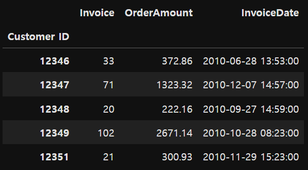
CustomerID 인덱스를 컬럼 값으로 변경 : reset_index()
customer_df = customer_df.reset_index()
customer_df.head()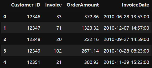
컬럼명 변경
Invoice -> Freq(주문횟수)
InvoiceDate -> ElapsedDays(마지막 주문일로부터 경과 일 수)
customer_df.rename(columns= {'Invoice': 'Freq', 'InvoiceDate': 'ElapsedDays'}, inplace= True)
마지막 주문일로부터 기준일까지 경과된 일수 계산
식 = 기준일 - 마지막 구매일 (기준일: 2011년 9월 12일(원본데이터 수집기간: 2009.1.12 ~ 2011.9.12))
datetime으로 만들어서 산술계산이 가능해지게 만든 후
customer_df['ElapsedDays'] = pd.to_datetime('2011.9.12') - customer_df['ElapsedDays']시간은 따로 필요가 없는 사항이기 때문에 .days를 통해 날짜만 추출한다.
# 일자만 나오게
customer_df['ElapsedDays'] = customer_df['ElapsedDays'].apply(lambda x: x.days)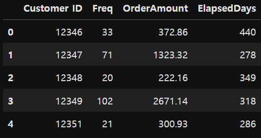
데이터 분포 확인
import matplotlib.pyplot as plt

fig, ax = plt.subplots()
ax.boxplot([customer_df['Freq'],customer_df['OrderAmount'],customer_df['ElapsedDays']], sym = 'bo')
plt.xticks([1,2,3],['Freq','OrderAmount', 'ElapsedDays'])
plt.show()

# 서로 데이터 분포가 다르기 때문에  같은 비율로 보이게 해야함 -> 스케일링 필요
# logscailing : 큰 숫자를 같은 비율로 보이게 해주어 데이터 분포를 고르게 해줌
집계 함수를 제각각 설정해주었기 때문에, 데이터의 분포가 맞지 않다 >> 로그로 변환시켜 데이터의 크기를 맞춘다.

데이터 로그변환
로그를 취해주게 되면 큰 숫자를 같은 비율의 작은 숫자로 만들어준다. 왜도와 첨도가 줄어들면서 정규성이 높아진다.
- 왜도 (Skewness , 비대칭 정도) : 평균에 대해 분포의 비대칭 정도를 나타내는 지표
- 첨도 (Kurtosis , 분포의 뾰족한 정도) : 관측치들이 어느정도 집중적으로 중심에 몰려있는가를 나타내는 지표
customer_df['Freq_log'] = np.log1p(customer_df['Freq'])
customer_df['OrderAmount_log'] = np.log1p(customer_df['OrderAmount'])
customer_df['ElapsedDays_log'] = np.log1p(customer_df['ElapsedDays'])
customer_df.head()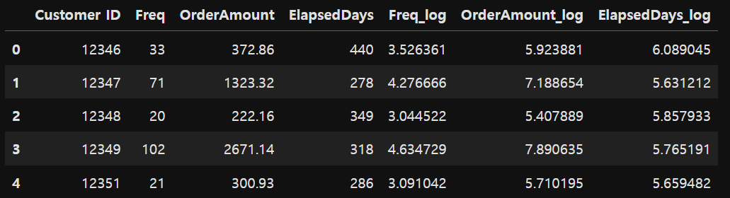
fig, ax = plt.subplots()
ax.boxplot([customer_df['Freq_log'],customer_df['OrderAmount_log'],customer_df['ElapsedDays_log']], sym = 'ro')
plt.xticks([1,2,3],['Freq_log','OrderAmount_log', 'ElapsedDays_log'])
plt.show()
데이터의 분포가 정규화된 것을 알 수 있다.

모델 생성
1. 최적의 K 찾기 - elbow function 이용
k_range = range(1,10) - > k의 값을 점차 증가시키며 학습시킨다.
x = customer_df[['Freq_log','OrderAmount_log','ElapsedDays_log']]from sklearn.cluster import KMeans
inertia_arr = []
k_range = range(1,10)
for k in k_range:
kmeans = KMeans(n_clusters=k, random_state= 10)
kmeans.fit(x) # 학습
inertia_arr.append(kmeans.inertia_)
# Elbow function 그리기
plt.plot(k_range, inertia_arr, marker = 'o')
plt.xlabel('Number of Clusters')
plt.ylabel('Inertia')
plt.show()
군집에서 적절한 k 의 값은 3 또는 4일 것이라고 예상된다.
2. 최적의 K 찾기 - 실루엣 계수 이용
visualize_silhouette([2,3,4,5,6],x)
최적 k를 이용한 군집분석 (최적의 k를 4로 결정)
model 을 내가 정한 k의 값으로 학습 시킨다.
best_k = 4
model = KMeans(n_clusters= best_k)
model.fit(x) # 스케일링한 데이터

cluster = model.labels_
model.labels 정답을 cluster 변수에 저장시킨 후 원본 데이터에 넣는다.
customer_df['cluster'] = cluster
print(np.unique(cluster))
customer_df.head()
[0 1 2 3]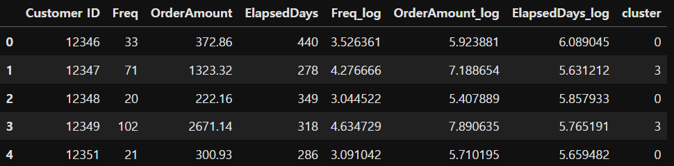
군집 분석 결과 시각화
시각화를 위해 아까 만들어 놓은 지수 함수로 만들어진 컬럼을 넣은 변수 x에 정답을 넣는다.
x['cluster'] = model.labels_
for i in range(best_k):
    plt.scatter(x[x['cluster']==i]['Freq_log'],
                x[x['cluster'] == i]['OrderAmount_log'],
                label = 'cluster-'+str(i))

plt.plot(model.cluster_centers_[:,0], model.cluster_centers_[:,1], 'bx', label = 'cluster center')
plt.legend()
plt.show()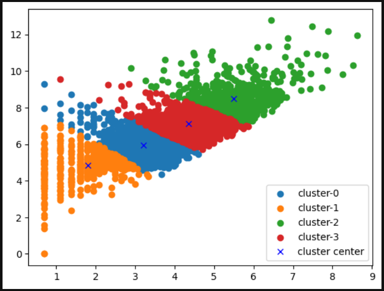
군집 결과 의미 해석
# 실제 데이터를 가지고 군집을 해석해야 한다.
customer_df_cluster = customer_df[['Freq','OrderAmount','ElapsedDays','cluster']]
customer_df_cluster.head()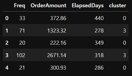
구매 1회당 평균 구매 비용 컬럼 추가
customer_df_cluster['OrderAmount_avg'] = customer_df_cluster['OrderAmount']/ customer_df_cluster['Freq']
그룹별 레코드 개수 확인
groupby_cluster = customer_df_cluster.groupby('cluster')
groupby_cluster['Freq'].count()
cluster
0 1541
1 603
2 726
3 1444
Name: Freq, dtype: int64groupby_cluster.mean()
>>> 0번째와 1번째 고객을 비교함으로써 많이 구매한 고객이 유효한 실적을 내는 것은 아니라는 것을 확인할 수 있었다.
'국비 교육 > 머신러닝, 딥러닝' 카테고리의 다른 글
| [머신러닝] 인공지능을 위한 수학(3. 선형대수) (0) | 2023.11.27 |
|---|---|
| [머신러닝] 비지도 학습 알고리즘 - 주성분분석(공분산행렬) - 1 (0) | 2023.11.26 |
| [머신러닝] 비지도 학습 알고리즘 - 군집분석 : K- 평균 군집 (0) | 2023.11.23 |
| [머신러닝] [문제] 비행기 연착 추측 분류 (0) | 2023.11.23 |


